SCRIN: Subcellular Colocalized RNA Interaction Network

SCRIN is a tool for identifying RNA co-localization networks within subcellular spatial transcriptomics data. While traditional co-localization methods are often bottlenecked by the scale of high-throughput data, SCRIN is engineered for unprecedented speed and memory efficiency, unlocking large-scale spatial transcriptomics analysis that was once computationally prohibitive.

Quick Start

To run SCRIN with the example dataset:

1. Install SCRIN and its dependencies following Installation.
2. Download the example dataset from Zenodo. The workflow uses Mouse_brain_CosMx_787cells.csv.
3. Check that the CSV follows the required Input Data Format.
4. Run the command in Examples, then inspect the files described in Step 3.

Requirements & Compatibility

The following dependencies are required to run this project. The versions listed have been tested thoroughly and confirmed to be compatible.

In most cases, other versions also work, as the project relies mainly on stable and widely supported APIs. If you encounter issues, we recommend reverting to the specified versions.

Note: This project has been tested and is currently supported only on Linux. Support for Windows and macOS may be added in the future, but compatibility is not guaranteed at this time.

Tested Environment:

• Python 3.9
• Linux

System Dependencies

• MPICH (== 4.2.1): Required for parallel computing. SCRIN utilizes high-speed parallel processing to efficiently handle large-scale spatial transcriptomics data.

Python Dependencies

• mpi4py==3.1.5
• msgpack==1.1.1
• numpy==2.0.2
• pandas==2.3.1
• pyarrow==21.0.0
• rtree==1.4.0
• scikit-learn==1.6.1
• scipy==1.13.1
• statsmodels==0.14.5
• tqdm==4.67.1

Installation

Step 1: Set up Python Environment

We recommend using Anaconda to manage your environment. Create and activate a new environment:

conda create -n scrin_env python=3.9
conda activate scrin_env

Step 2: Install MPICH

SCRIN leverages mpi4py for high-speed parallel computing to tackle the challenges of large-scale spatial transcriptomics data. This requires a functional MPI (Message Passing Interface) implementation on your system, such as MPICH.

Please install MPICH using one of the following methods before proceeding.

Method 1: Install via Conda

The easiest way to ensure compatibility is to let Conda install mpi4py and its required MPI implementation (MPICH) together.

conda install -c conda-forge mpi4py=3.1.5 mpich=4.2.1

Note on Version Availability: If the command above fails because the specified versions cannot be found for your system, you can try installing without specifying the versions:

conda install -c conda-forge mpi4py mpich

Please be aware that this will install the latest available packages, which have not been officially tested by us and may lead to unexpected behavior.

Method 2: Install via System Package Manager

For Debian-based systems like Ubuntu, you can use apt:

sudo apt update
sudo apt install mpich=4.2.1

Method 3: Install from Source

For advanced users or specific system configurations, you can compile and install MPICH from the official source. Please refer to the official MPICH installation guide for detailed instructions.

Step 3: Install Python Dependencies

Before installing SCRIN, install the dependencies listed in requirements.txt:

pip install -r requirements.txt

Note: If you did not use the Conda method to install MPICH in Step 1, pip will attempt to compile mpi4py using the system's MPI compiler (mpicc). Ensure your MPICH installation is correctly configured in your system's PATH.

Step 4: Install SCRIN

Once dependencies are installed, SCRIN can be installed in two ways:

1. Install from PyPI

To install the latest stable release:

pip install scrin

The 1.1.0rc3 pre-release provides early access to the new downstream analysis modules and performance optimizations planned for SCRIN 1.1:

pip install --upgrade scrin==1.1.0rc3

Because 1.1.0rc3 is a pre-release, it is not selected by the default pip install scrin command when a stable release is available.

2. Install from local clone

git clone https://github.com/xryanglab/SCRIN
cd SCRIN
pip install .

Usage

The basic command structure to run SCRIN is as follows:

mpirun -n <number_of_processes> scrin [OPTIONS]

Input Data Format

SCRIN expects a CSV (Comma-Separated Values) file as input. The file should contain columns for spatial coordinates (x, y, and optionally z), a gene identifier, and a cell identifier. The header names can be arbitrary, as they will be mapped using the --column_name parameter.

Here are the first few lines of the example dataset on Zenodo, Mouse_brain_CosMx_787cells.csv:

x,y,z,gene,cell
-55407.27163461538,1496.6466346153845,-1,Sparcl1,98_241
-55403.90625,1498.0685096153845,0,Ntrk2,98_241
...

Column requirements:

• Coordinates (x, y, z): At least x and y columns are required. The z column is optional. Spatial parameters such as --r_check and --r_dist must use the same unit as the coordinates; the example dataset x/y coordinates are in micrometers.
• Gene ID (gene in the example dataset): A column containing the names or identifiers of the RNA species.
• Cell ID (cell in the example dataset): A column indicating which cell each transcript belongs to. This is highly recommended for standard analysis. For data without pre-existing cell segmentation, please refer to the Unsegmented Data Options.

Note: Some input files may include extracellular transcripts, often indicated by a cell ID value that does not correspond to a segmented cell. If you plan to use --background "cooccurrence", these transcripts should be removed before running SCRIN. If you use --background "all", keep these transcripts only if you want to include them in the global background statistics; otherwise, remove them before running SCRIN.

Examples

Step 1: Download the example dataset

This workflow uses a spatially contiguous, approximately 500 × 500 µm region containing 787 cells, derived from the CosMx SMI Mouse Brain FFPE dataset by NanoString. The sampled field approximately corresponds to the dentate gyrus (DG) region of the mouse hippocampus. The x/y coordinates have been converted from pixels to micrometers, allowing both the main SCRIN analysis and tissue-level downstream visualization.

Example dataset: Download the ready-to-run Mouse_brain_CosMx_787cells.csv file from Zenodo. Direct URL: https://zenodo.org/records/21486759

Compact derived outputs, plotting inputs, scripts, and figures are available in the repository's 787-cell mouse-brain example.

Step 2: Run the main SCRIN analysis

# Launch SCRIN on 16 parallel processes. Adjust the value of -n as needed.
mpirun -n 16 scrin \
	--detection_method "radius" \
	--background "cooccurrence" \
	--mode "fast" \
	--data_path "Mouse_brain_CosMx_787cells.csv" \
	--save_path "Mouse_brain_CosMx_787cells_hyper_result_cb.csv" \
	--column_name "x,y,z,gene,cell" \
	--r_check 0.5 \
	--z_mode "discrete" \
	--filter_threshold 0.00001 \
	--min_gene_number 5 \
	--min_neighbor_number 1 \
	--expression_level 100 \
	--intermediate_dir "Mouse_brain_CosMx_787cells_hyper_result_cb"

Explanation of parameters:

• --detection_method "radius": Since CosMx data provides continuous spatial coordinates, we use the radius method to define neighbors based on their straight-line distance.
• --background "cooccurrence": The mouse brain is a highly heterogeneous tissue containing many different cell types. Using cooccurrence is recommended here, as it calculates the statistical background for a gene pair (A-B) using only the cells where both A and B are expressed. This provides a more specific and relevant context compared to the all option (which would be suitable for more homogeneous samples like single cell type). When using this option, remove extracellular transcripts or transcripts not assigned to any cell from the input CSV.
• --mode "fast": We use the fast mode to enable high-speed, low-memory parallel processing, which is essential for large datasets. This requires an intermediate directory (--intermediate_dir) to store temporary files.
• --data_path: Specifies the location of your input raw data. The required CSV structure is described in the Input Data Format section.
• --save_path: The file path where the co-localization results will be saved.
• --column_name: This parameter maps the input columns (x, y, z, gene, and cell) to the fields SCRIN expects, as described in the Input Data Format section.
• --r_check 0.5: Sets a 0.5 µm search radius because the example dataset x/y coordinates are already expressed in micrometers.
• --z_mode "discrete": Since CosMx data consists of several discrete z-planes that are relatively far apart, we use the discrete mode to ensure neighbor searching only occurs within the same imaging plane.
• --filter_threshold 0.00001: Sets the q-value cutoff for the final results, ensuring that only statistically significant interactions are reported.
• --min_gene_number 5: A pre-filtering step to improve efficiency by excluding sparsely expressed genes (those with fewer than 5 total transcripts in the dataset) from the analysis.
• --min_neighbor_number 1: Skips significance testing for gene pairs with zero observed co-localization events, as they cannot be statistically significant.
• --expression_level 100: Filters out gene pairs with highly imbalanced expression levels (where one gene's transcript count is over 100 times that of the other) to avoid potential artifacts.
• --intermediate_dir: Specifies the directory to store temporary files during parallel processing. This is required when running in fast mode to manage memory efficiency across multiple processes.

Step 3: Inspect the expected output

After completion, SCRIN produces two main output files:

• Raw output: Mouse_brain_CosMx_787cells_hyper_result_cb.csv
• Final processed output: Mouse_brain_CosMx_787cells_hyper_result_cb_dedup_1e-05_post_proc.csv

The final processed output contains significant RNA co-localization pairs after q-value filtering and bidirectional pair deduplication. Key columns include gene_A, gene_B, qvalue_BH, enrichment_ratio, and support_ratio. See the Output section below for the full column descriptions and an example result snippet.

Step 4: Explore downstream analyses and visualizations

The main SCRIN workflow can be followed by optional downstream analyses, visualizations, and diagnostic evaluations. The downstream commands below require SCRIN 1.1.0rc3 or a current installation from the GitHub repository.

• Colocalization Distance-distribution Analysis must be enabled during the original SCRIN run using the distribution-analysis options because transcript-pair distances are collected during neighborhood detection.
• Cell-level Colocalization Events for Tissue Projection can be performed afterward for selected pairs using scrin-colocalization-events and the original transcript-coordinate file, without rerunning the main significance-testing workflow.
• Empirical False-positive Baseline Analysis evaluates control-associated pairs across q-value thresholds using the raw SCRIN result.
• Multi-radius Analysis of Colocalization Scale compares pair significance across neighborhood radii to examine scale-dependent colocalization patterns.

Derived data, plotting scripts, and figures for the visualization examples are available in the 787-cell mouse-brain example.

Command-line Options

Mode Options

• --detection_method [radius|nine_grid] (Required): Method for defining neighboring transcripts.

  • radius: Defines neighbors based on the straight-line distance between transcripts. Any transcript within the distance specified by --r_check is considered a neighbor. This is suitable for continuous-coordinate data, such as from MERFISH.
  • nine_grid: Defines neighbors as any transcripts located within the same grid square or its eight adjacent squares. This is suitable for array-based data with orderly coordinates, such as from Stereo-seq.

• --background [all|cooccurrence] (Required): Define the statistical scope used to calculate the parameters for the hypergeometric test.

  • all: All cells in the dataset are used to calculate the background parameters (n, M, N). For each gene, these parameters are computed only once, enabling more consistent comparison of colocalization strength across gene pairs and higher computational efficiency. This option is useful for homogeneous datasets, rapid exploratory analyses, or applications where a common global background is preferred for detecting weaker colocalization signals.
  • cooccurrence: For a given gene pair A-B, only cells where both A and B are present are used to calculate the background parameters. This pair-specific background generally provides more specific and reliable results by excluding cells that are not informative for the tested pair, including in relatively homogeneous datasets. It is therefore recommended for most analyses, particularly for heterogeneous datasets containing mixed or highly specific cell types, although it has a higher computational cost than all. When using this mode, ensure that transcripts not assigned to any cell (extracellular noise) are removed from your input CSV; see the Input Data Format section.
  • Note: The value k (observed co-localizations) is calculated the same way in both modes, but the background parameters n, M, and N will differ.

• --mode [robust|fast] (Required): The running mode for the program.

  • fast: Uses the optimized implementation for large-scale datasets. For the cooccurrence background, it exchanges compact K/R records in explicit MPI batches and reconstructs background statistics by gene-A row, without the legacy per-cell Cartesian updates or complete five-channel matrix gathering.
  • robust: Uses the stable reference implementation. It requires more memory and is suitable for small validation runs or direct comparison with fast mode.

Base Parameters

• --data_path [str] (Required): Path to the input data file. The file must contain transcript spatial coordinates and gene IDs at a minimum. Including cell IDs is recommended. Please refer to the Input Data Format section and the example dataset, Mouse_brain_CosMx_787cells.csv, for the standard input format.
• --save_path [str] (Required): Path for saving the results.
• --column_name [str] (Required): A comma-separated string specifying which columns from the input file to use. The provided names are mapped sequentially to the expected fields described in the Input Data Format section: x (x-coordinate), y (y-coordinate), z (z-coordinate, optional), geneID (gene ID), and cell (cell ID, optional). If an optional field like z is not present in your data, simply omit it from the string while maintaining the order of the remaining fields. For example, if your file provides columns for x, y, geneID, and cell (but no z), and their names are pos_x, pos_y, gene_name, cell_label, your input should be "pos_x,pos_y,gene_name,cell_label". The minimum required fields correspond to x, y, and geneID. Default: "x,y,z,geneID,cell".
• --r_check [float ...]: One or more search radii for the 'radius' detection method. Transcripts with a distance less than or equal to a radius are considered neighbors. When multiple values are provided, SCRIN runs the complete analysis once per radius in ascending order. Per-radius result files receive an _r_<radius> suffix, and per-radius intermediate files are stored in separate subdirectories under --intermediate_dir. A single value preserves the original output paths.
• --z_mode [discrete|continuous]: Specifies how the vertical dimension (z-axis) is handled during neighbor searching. Default: discrete.
  • discrete: Neighbors are only searched within the same z-plane. This mode is designed for datasets where z-planes are relatively far apart compared to the search radius, or when co-localization is expected to occur only within the same imaging plane (e.g., MERFISH or CosMx data). Note: If your data lacks z-coordinates entirely, you should use this mode.
  • continuous: Uses Euclidean distance across x, y, and z. Use this mode only after confirming that the z coordinates and their scale are appropriate for direct 3D distance calculations; otherwise, use discrete.
• --grid_check [int]: Sets the search window size for the 'nine_grid' method. It defines a square area of (2 * grid_check + 1) x (2 * grid_check + 1) grid cells around a central transcript. For example, grid_check=1 defines a 3x3 grid (9 cells), while grid_check=2 defines a 5x5 grid (25 cells). Transcripts within this area are considered neighbors.
• --min_gene_number [int]: A pre-filtering step to remove sparsely expressed genes. Any gene whose total transcript count across the entire dataset is below this value will be excluded from the analysis. Default: 5.
• --min_neighbor_number [int]: Filters out gene pairs with insufficient co-localization events. For a given pair A-B, if the number of times transcripts of gene B are detected as neighbors of transcripts of gene A is below this threshold, that pair will be skipped during the significance calculation. Default: 1.
• --expression_level [float]: A filter to exclude gene pairs with highly imbalanced expression. This value sets the maximum allowable fold-difference in total transcript counts between two genes. For example, with the default of 100, any pair where one gene is over 100 times more abundant than the other will be ignored. Default: 100.
• --filter_threshold [float]: The q-value (Benjamini-Hochberg adjusted p-value) threshold for filtering results in post-processing. Default: 0.00001.
• --pair_keep [first|last]: Method for deduplicating bidirectional pairs (e.g., A-B and B-A) during post-processing. Pairs are first sorted by their q-value in ascending order. first keeps the pair with the smaller q-value, while last keeps the one with the larger q-value. Default: 'last'.

Intermediate Result Options

For large datasets, use these options to save intermediate results and prevent memory overflow.

• --intermediate_dir [str]: Directory path to save intermediate results. This parameter is required when using fast mode.
• --intermediate_split [int]: Controls the chunk size for processing. A larger value reduces memory usage but may decrease computational efficiency. It is not recommended to set this value higher than the total number of genes or 1000, as excessive partitioning can lead to issues. Default: 100.

Distribution Options

Options for analyzing the distance distribution of co-localized gene pairs.

• --distribution_analysis: A flag to enable the analysis. This will save the distance distribution for each neighboring pair and calculate its statistical features. Warning: This can generate very large files and significantly increase runtime. Ensure you have sufficient disk space before enabling.
• --r_dist [float]: Defines the maximum radius for the distance distribution analysis. For a pair A-B, transcript-pair distances less than or equal to this value are recorded.
• --around_count_threshold [int]: Minimum number of transcript-pair distances required to calculate distribution-shape statistics for a gene pair. Distances are pooled across cells, and the code uses shape_count >= around_count_threshold. Default: 100.
• --shape_max_distance_count [int]: Maximum number of distances used to calculate shape descriptors for each pair. When the original shape_count exceeds this value, SCRIN uses a reproducible random sample for KDE mode and the other descriptors while retaining the full distance data in the intermediate files. shape_count continues to report the original number of distances. Default: 10000. Users may lower the value for faster analysis or increase it when greater descriptor stability is preferred; the value must be at least around_count_threshold.
• --shape_qvalue_threshold [float]: Only directed pairs with qvalue_BH below this threshold are considered for shape calculation, substantially reducing unnecessary KDE calculations. Default: 0.05, providing broad coverage of potentially relevant pairs. Use a value at least as large as filter_threshold when shape descriptors are desired for every final pair.
• --distribution_save_interval [int]: For the cooccurrence background, controls how often worker-side distance data is written to intermediate files. A smaller value reduces worker memory usage but increases file I/O. This parameter is not used by the all-background distribution path. Default: 10.

Unsegmented Data Options

For data without prior cell segmentation.

• --unsegmented: A flag to enable processing of unsegmented data.
• --rect_length [float]: The side length of the rectangle used to partition the data. The recommended value is the approximate cell diameter. Default: 20.
• --rtree_path [str]: Path to an R-tree index file for accelerating spatial queries. If not specified (None), the index is built in memory. If a path is provided but the file doesn't exist, a new index will be built and saved there; if it exists, it will be loaded to accelerate queries.

Output

SCRIN generates two main types of output files: a raw results file and a post-processed file for downstream analysis.

Final Processed Output

This is the primary result file you will typically use. It is generated by performing several post-processing steps on the raw output. For the example command, this file would be named Mouse_brain_CosMx_787cells_hyper_result_cb_dedup_1e-05_post_proc.csv.

The post-processing includes:

1. Adding a pair column: A standardized, sorted identifier for each gene pair (e.g., GeneA_GeneB) is added to facilitate deduplication.
2. Calculating the Enrichment Ratio: An enrichment ratio is calculated to prioritize pairs with a higher degree of enrichment.
3. Calculating the Support Ratio: A support ratio is calculated to prioritize pairs with stronger event-level support independent of statistical significance.
4. Sorting: The results are sorted by the Benjamini-Hochberg adjusted q-value (qvalue_BH) in ascending order.
5. Deduplication: Bidirectional pairs (e.g., A-B and B-A) are deduplicated based on the --pair_keep parameter.
6. Filtering: The results are filtered to keep only the interactions with a qvalue_BH below the --filter_threshold.

An example snippet from the final output file is shown below:

gene_A,gene_B,pvalue,qvalue_BH,qvalue_BO,gene_B_around,gene_B_slice,gene_around,gene_slice,gene_A_N,gene_B_N,pair,enrichment_ratio,support_ratio
Clu,Apoe,3.546414862528735e-170,2.6172541685462066e-167,2.6172541685462066e-167,451,5932,9697,643013,3729,5932,Apoe_Clu,5.04147661674009,0.12094395280235988
...

Basic Filtering Recommendations

SCRIN's final output contains statistically significant colocalization pairs after directional deduplication and q-value filtering. Whole-transcriptome datasets may still contain many weak but detectable spatial associations, so additional filtering can help prioritize pairs for downstream analysis.

A permissive starting point is:

gene_B_around >= 10
support_ratio >= 0.01

These cutoffs are intentionally lenient rather than universal. Thresholds for gene_B_around, support_ratio, enrichment_ratio, qvalue_BH, and other relevant metrics can be adjusted according to the dataset, platform, and biological question.

Raw Output

The program also saves the raw, unfiltered results from the hypergeometric test. Using the example command, this file would be Mouse_brain_CosMx_787cells_hyper_result_cb.csv. This file contains all calculated gene pairs before any sorting, deduplication, or q-value filtering, and can be useful for custom analyses or diagnostics.

Column Descriptions

The columns in the output files correspond to the standard parameters of a hypergeometric test and additional calculated metrics.

Column	Description
gene_A	The central gene in the pair.
gene_B	The target gene found in the neighborhood of the central gene (gene_A).
pvalue	The raw p-value calculated from the hypergeometric test.
qvalue_BH	The p-value adjusted for multiple testing using the Benjamini-Hochberg (BH) method. This is the primary value for assessing significance.
qvalue_BO	The p-value adjusted using the more conservative Bonferroni method.
gene_B_around	(k) The number of observed co-localizations: how many times transcripts of the target gene (gene_B) were found in the neighborhood of the central gene (gene_A).
gene_B_slice	(M) The total number of target gene (gene_B) transcripts within the defined statistical background.
gene_around	(n) The total number of all transcripts (from any gene) found in the neighborhood of the central gene (gene_A).
gene_slice	(N) The total number of all transcripts in the defined statistical background.
gene_A_N	The total transcript count for the central gene (gene_A) in the defined statistical background.
gene_B_N	The total transcript count for the target gene (gene_B) in the defined statistical background; same as gene_B_slice.
pair	A standardized identifier for the gene pair (e.g., alphabetically sorted), used for post-processing.
enrichment_ratio	Neighborhood enrichment relative to the statistical background, calculated as (gene_B_around / gene_around) / (gene_B_slice / gene_slice). It helps prioritize pairs with stronger enrichment.
support_ratio	Event-level support normalized by the less abundant transcript count, calculated as gene_B_around / min(gene_A_N, gene_B_N). It provides an intuitive measure of colocalization-event support independent of statistical significance.

Downstream Analysis Tools

The downstream tools documented below are available in the 1.1.0rc3 preview release. See Install from PyPI for the explicit installation command.

The following independent commands provide optional downstream analyses and do not rerun or alter the main SCRIN workflow.

Colocalization Distance-distribution Analysis

Distance-distribution analysis must be enabled during the original SCRIN run because the raw transcript-pair distances are collected during neighborhood detection. It is available for segmented data in fast, radius, and discrete z mode. Add the following options to a standard SCRIN command:

--distribution_analysis \
--r_dist 1.0 \
--around_count_threshold 100 \
--distribution_save_interval 10

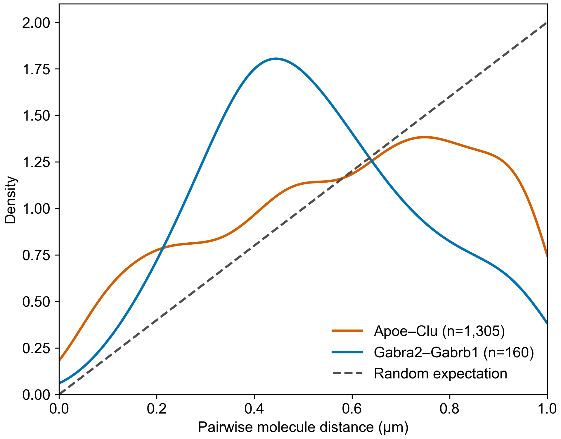
r_check defines the neighborhood used by the colocalization test, whereas r_dist defines the distance range retained for distribution analysis. We recommend setting r_dist larger than r_check so the distribution also shows distances beyond the colocalization boundary; using the same value truncates that side of the curve and can make its shape difficult to interpret. For the example dataset, r_check=0.5 µm and r_dist=1.0 µm. Distance observations are collected within cells and within the same z-plane.

For --save_path result.csv, the principal outputs are:

result.csv
result_shape.csv
result_dedup_<filter_threshold>_post_proc_shape.csv

result_shape.csv contains directed intermediate summaries for pairs that pass shape_qvalue_threshold and have at least around_count_threshold distances. The final post_proc_shape file applies SCRIN's final q-value filtering and undirected pair deduplication, then joins the shape statistics. Significant pairs excluded by the shape q-value or distance-count threshold remain in the final file with missing shape values.

shape_count is the number of transcript-pair distance observations pooled across cells for a q-value-eligible pair; shape descriptors additionally require shape_count >= around_count_threshold. The other shape columns include KDE-estimated mode, skewness, excess kurtosis, median, q25, q75, and iqr, while skewness_adjusted = 1 / (1 + exp(skewness)) maps skewness to a 0-1 scale. These descriptors provide a quick overview of distribution shape and help screen pairs for closer inspection. The *_relative columns report the observed-minus-reference shift after subtracting this geometric background, making the direction of the distribution bias easier to interpret; for example, negative relative quantiles indicate a shift toward shorter distances.

The actual distance lists remain in the retained intermediate directory. Extract one or more undirected pairs without rerunning SCRIN:

scrin-extract-distances \
	--intermediate_dir "Mouse_brain_CosMx_787cells_hyper_result_cb" \
	--pair "Apoe" "Clu" \
	--pair "Gabra2" "Gabrb1" \
	--min_distance_count 50 \
	--max_distance_count 10000 \
	--random_seed 42 \
	--save_path "selected_pair_distances.parquet"

A-B and B-A have the same distance distribution and are treated as one undirected pair. Reversed or repeated inputs are consolidated. For many pairs, use --pair_path with a CSV file containing either gene_A and gene_B columns:

gene_A,gene_B
Apoe,Clu
Gabra2,Gabrb1

The alternative headers gene_1 and gene_2 are also accepted. Additional columns are ignored, so a SCRIN result CSV can be supplied directly. Use the file with --pair_path "pairs.csv"; --pair_path and --pair cannot be used together.

--min_distance_count discards pairs with fewer observations. When a pair has more than --max_distance_count, the command takes a reproducible uniform sample without replacement; pairs within the requested range are exported completely. Defaults are min_distance_count=1 and no maximum, so extraction is lossless unless sampling is explicitly requested. Sampling can reduce output size and make distribution plotting more manageable.

Output paths ending in .csv, .csv.gz, and .parquet are supported. Parquet is recommended for large outputs. The long-form output contains gene_1, gene_2, pair, and distance; distance uses the same coordinate unit as the input x/y values. A companion *_summary.csv records the original count, exported count, and whether each pair was complete, sampled, below the minimum, or not found.

For an ideal random reference, suppose B transcripts are uniformly distributed in a complete two-dimensional disk of radius (R) around A. Conditional on (0 \le r \le R), the radial distance has:

PDF: f(r) = 2r / R^2
CDF: F(r) = r^2 / R^2

The PDF follows from the increasing area of an annulus at radius (r). Overlaying it on empirical KDE curves makes distance preferences easier to see: enrichment or a left shift toward short distances indicates stronger short-range organization, whereas a curve closer to the random reference is more consistent with broader co-compartment localization.

The repository example compares Apoe-Clu and Gabra2-Gabrb1 using the extracted distance data and plotting script. Gabra2-Gabrb1 shows a stronger short-distance preference, while Apoe-Clu has a broader profile.

Cell-level Colocalization Events for Tissue Projection

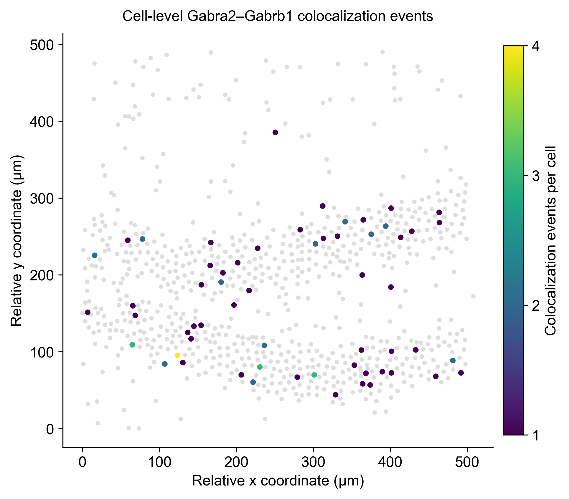
The independent scrin-colocalization-events command quantifies selected undirected gene-pair signals at single-cell resolution for projection back onto tissue space. For an undirected pair A-B, every transcript-level A-B connection with a distance less than or equal to --r_check contributes one colocalization event. The total number of such connections in each cell provides a direct measure of the local abundance of spatially proximal A-B transcript pairs.

The command recalculates event counts from the original transcript coordinates for only the requested pairs and reports them together with representative cell coordinates. These cell-resolved values can be mapped to colors or other visual encodings in tissue plots without rerunning the main SCRIN significance-testing workflow.

To calculate one pair:

scrin-colocalization-events \
	--data_path "Mouse_brain_CosMx_787cells.csv" \
	--save_path "Gabra2_Gabrb1_cell_events.csv" \
	--column_name "x,y,z,gene,cell" \
	--pair "Gabra2" "Gabrb1" \
	--r_check 0.5 \
	--z_mode "discrete" \
	--n_jobs 8

For multiple pairs, supply --pair_path instead of --pair. The pair file must contain gene_A and gene_B columns. A SCRIN result CSV can be used directly because additional columns are ignored. Bidirectional and repeated pairs are consolidated, while self-pairs such as A-A are not supported.

The output contains one row per cell and requested pair, including cells with zero events:

cell,cell_x,cell_y,gene_A,gene_B,r_check,gene_A_count,gene_B_count,colocalization_count
99_211,-55310.9375,1292.1442307692307,Gabra2,Gabrb1,0.5,9,8,1

cell_x and cell_y are the coordinate-wise medians of all transcripts in the cell, including genes outside the requested pairs. For tissue projection, the input transcript x/y values must be global tissue coordinates. If the input uses coordinates local to each cell or field, these medians will not represent the cells' positions in the full tissue. gene_A_count and gene_B_count are the corresponding transcript counts in that cell. Duplicate transcript rows are retained as separate molecules. With --z_mode discrete, only transcripts in the same z-plane can form an event; with --z_mode continuous, three-dimensional Euclidean distance is used.

Use cell to link the result to cell metadata or segmentation boundaries, and use cell_x, cell_y, and colocalization_count to draw a point-based tissue map or to color cell regions by event count. Such projections can reveal where an undirected colocalization pair is concentrated across the tissue, including spatial gradients, regional enrichment, or localized hotspots.

The provided Gabra2-Gabrb1 event table and plotting script produce the map below.

--n_jobs controls local multiprocessing and defaults to 1. Increase it to process cells in parallel.

Empirical False-positive Baseline Analysis

Platform-provided negative-control features can be used to examine whether control-associated background contributes to SCRIN-detected colocalization pairs. The example dataset contains ten negative-control probes named NegPrb1 through NegPrb10. Analyze them with:

scrin-false-positive-analysis \
	--result_path "Mouse_brain_CosMx_787cells_hyper_result_cb.csv" \
	--control_group "negative_control_probe" "prefix" "NegPrb"

This command requires the raw SCRIN result rather than a threshold-filtered post_proc file. It reproduces SCRIN's bidirectional pair deduplication and then reports results at qvalue_BH < 0.05, 0.01, 0.001, and 1e-5 by default. Use --qvalue_thresholds to supply other cutoffs and --pair_keep when the original analysis used a non-default deduplication setting.

A pair is control-associated when either gene_A or gene_B matches a control rule. The reported control-associated pair fraction is:

number of significant control-associated pairs / total number of significant pairs

The fraction is an empirical diagnostic, not a direct estimate of the statistical false-positive rate or BH false discovery rate. It reflects only the background represented by the supplied control features and may depend on panel composition, control-feature abundance, and the number of control features.

Control rules use the form GROUP_NAME MATCH_MODE PATTERN. The same framework can be applied to user-provided synthetic decoy transcripts, provided that they follow a recognizable naming pattern and are specified as a separate control group. Supported match modes are exact, prefix, suffix, and contains; add --ignore_case for case-insensitive matching. Repeat --control_group to define multiple rules or groups. Each group is reported separately, and an any_control union is also reported when multiple groups are present.

Results are printed to the terminal. Use --save_path to additionally save the small summary table as CSV.

Multi-radius Analysis of Colocalization Scale

The neighborhood radius defines the spatial scale at which SCRIN evaluates transcript proximity. Smaller radii, approximately 0.2-0.5 µm, are useful starting points for highly local RNA organization, whereas larger radii, approximately 1-2 µm, can capture broader subcellular domains or compartment-level organization. These ranges are not universal: radius selection should reflect the biological question, the platform's spatial resolution, and the coordinate units of the input data.

With the radius detection method, provide multiple values after --r_check to run the complete SCRIN workflow at each radius. Because the example dataset coordinates are in micrometers, the desired radii can be supplied directly:

--detection_method "radius" \
--r_check 0.25 0.5 0.75 1.0 1.5 2.0

For --save_path result.csv, SCRIN creates radius-specific raw files such as result_r_0p25.csv and final files such as result_r_0p25_dedup_1e-05_post_proc.csv. Decimal points are represented by p in radius suffixes. When --intermediate_dir is supplied, each radius also receives a separate r_<radius> subdirectory using the same suffix format.

A common downstream analysis is to take the union of pairs significant at any radius, retrieve their qvalue_BH values from the raw result at every radius, and plot a pair-by-radius heatmap of -log10(qvalue_BH). This heatmap may reveal persistent, short-range, or broader-scale colocalization patterns across pairs.

Citation

If you use SCRIN in your research, please cite our publication.

For any questions, please contact:

Xuerui Yang (yangxuerui@tsinghua.edu.cn); Xu Chen (chenxu22@mails.tsinghua.edu.cn)